This is a followup to the Win Vector blog article Post-hoc Adjustment for Zero-Thresholded Linear Models, in which I showed how to use a one-variable GAM (e.g., a spline) to adjust a linear model in a problem space where outcomes are strictly nonnegative. If you haven’t read that article, I suggest you check it out, first.
Some Background #
The original motivation for the work we did here was to help a client who had built a fairly complex multivariate model to predict expected count data. Their underlying assumption was that in their domain, a count of zero is a rare event. To quote my previous article:
When you don’t expect to see too many zeros in practice, modeling the process as linear and thresholding negative predictions at zero is not unreasonable. But the more zeros (saturations) you expect to see, the less well a linear model will perform.
They then automated the model training and deployment process, and put it into production across multiple sites.
Unfortunately, zero-counts are not so rare as they originally believed, at some of their sites. Because coming up with and deploying a new model design is not necessarily feasible at this stage (at least not in the immediate term), they wanted to figure out how to adjust their existing models to operate even at high zero-count sites. Note that this adjustment is a one-dimensional process: mapping the output of one model to a prediction that is closer to the actual outcomes.
To motivate this adjustment process in the previous article, I used an example of a linear model that was fit to a one-dimensional saturated process. This was so I could plot the resulting “hockey stick” function, and show what happens with different model adjustments. But it’s been my experience that people won’t believe that this procedure will generalize to multivariate linear models, unless I show them that it works on such models. So in this article, I’ll apply the same procedures to a linear model that was fit to two variables, just to prove the point.
I’ll also add an additional adjustment that wasn’t in the original article, but was suggested by Neal Fultz: adjustment using a Tobit model. You can see more details of that in a revised version of the article on github, here. Tobit adjustments work nearly as well as GAM adjustments, and do have the (potential) advantage of having a stronger inductive bias, if you believe that your process is truly linear in its non-saturated regions [1].
In the second part of the article, I’ll try fitting a model directly to the input data, using both GAM and Tobit, since ideally, that’s what you’d do if you were approaching this modeling task de novo.
For legibility and brevity, I’m going to hide a lot of the code when generating this article, but you can find the original R Markdown source code on github as well, here.
Example Problem #
Here are the characteristics of our example problem:
- The feature
upositively correlates with outcome, whilevnegatively correlates. - The outcome
yis constrained to be nonnegative; in other words, it “saturates” at zero. - Both features
uandvare bounded between 0 and 1 uniformly. - There is a moderate noise process on top of it.
trueprocess = function(N) {
  u = runif(N)
  v = runif(N)
  noise = 0.3 * rnorm(N)
  y = pmax(0, 4 * u - 3 * v + noise)
  data.frame(u = u, v = v, y = y)
}
The Data #
Let’s generate some training data.
traind = trueprocess(1000)
head(traind)
## u v y
## 1 0.1634115 0.2125462 0.6570359
## 2 0.5249624 0.6152054 0.0000000
## 3 0.3051476 0.9153664 0.0000000
## 4 0.9277528 0.8064937 1.5395565
## 5 0.5715193 0.9990540 0.0000000
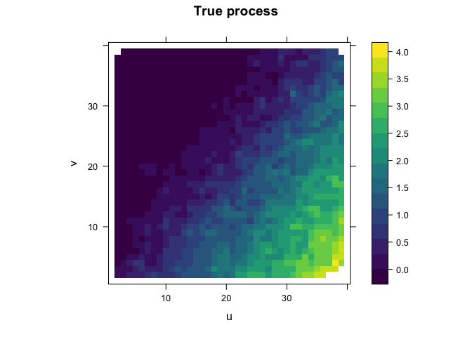
## 6 0.2602110 0.5206304 0.0000000Let’s plot a heatmap of the training data. Note that there’s lots of saturation.
We’re going to use all the data to train our models, but it’s not easy
to show comparison plots in three dimensions in a way that’s legible. So
we’ll also look at slices of the data, by holding u restricted to a
narrow range around a nominal value. Here’s a slice with u fixed to
near 0.5.
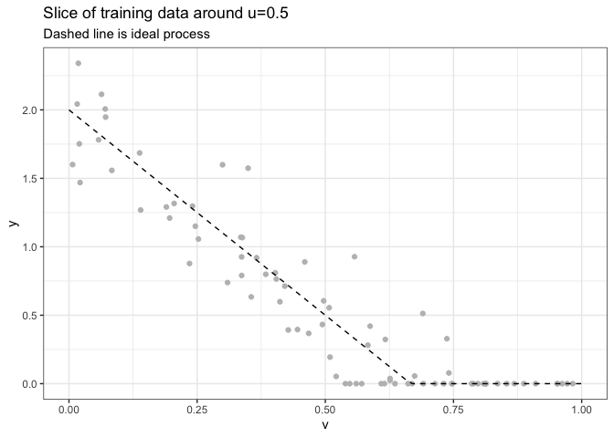
As you can see, the data is fairly noisy, in addition to being quite saturated. Now let’s train a linear model on the data, as well as all our adjusted models.
Part I: Adjustments to a Linear Model #
Train the initial model, and all the adjustments #
We’ll fit the model, make the naive adjustment of thresholding the data at zero, then fit all the candidate adjustment models. Note that only the initial model ever makes reference to the input variables.
# train the initial model,
# get the initial predictions and thresholded predictions

initial_model = lm(y ~ u + v, data=traind)
traind$y_initial= predict(initial_model, newdata=traind)
traind$y_pred0 = pmax(0, traind$y_initial)

# fit the adjustment models
# (function definitions in R markdown document)
scaling_model = fit_scaler(initial_model, "y", traind)
linadj_model = fit_linmod(initial_model, "y", traind)
gamadj_model = fit_gammod(initial_model, "y", traind)
tobitadj_model = fit_tobit(initial_model, "y", traind)

adjustments = list(scaling_model, linadj_model, gamadj_model, tobitadj_model)
names(adjustments) = c("y_linscale", "y_linadj", "y_gamadj", "y_tobitadj")

# make the predictions
for(adj in names(adjustments)) {
  traind[[adj]] = do_predict(adjustments[[adj]], newdata=traind)
}
Let’s look at the RMSE and bias of each model.
| prediction_type | description | RMSE | bias |
|---|---|---|---|
| initial | initial model | 0.4438901 | 0.0000000 |
| pred0 | zero-thresholded model | 0.3721101 | 0.0842275 |
| linscale | scale-adjusted model | 0.3692881 | 0.1196263 |
| linadj | linear-adjusted model | 0.2453422 | 0.0298617 |
| gamadj | GAM-adjusted model | 0.2261695 | 0.0007868 |
| tobitadj | Tobit-adjusted model | 0.2293762 | -0.0097394 |
Model RMSE and bias on training data
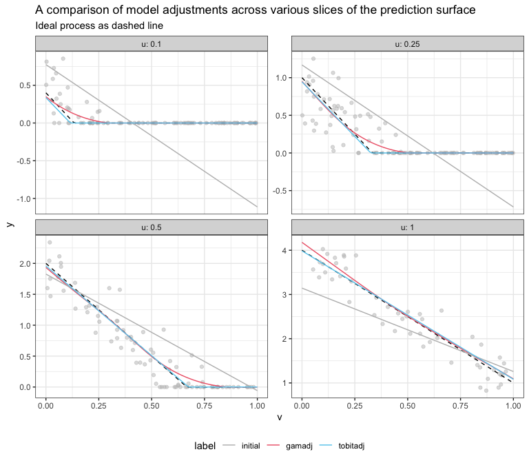
As expected (if you’ve read the previous article), the GAM-adjusted model has the lowest training RMSE, and also lower bias than the other adjusted models. The Tobit-adjusted model has comparable RMSE, and slightly more bias.
We can try to visualize what’s happening, by holding u constant at
different values and looking at slices of the prediction surfaces. We’ll
just compare the original linear model, GAM-adjustment, and
Tobit-adjustment.
Test on holdout #
Let’s compare the models on holdout data. For this example the holdout performances are similar to training.
testd = trueprocess(5000)

testd$y_initial= predict(initial_model, newdata=testd)
testd$y_pred0 = pmax(0, testd$y_initial)
for(adj in names(adjustments)) {
  testd[[adj]] = do_predict(adjustments[[adj]], newdata=testd)
}| prediction_type | description | RMSE | bias |
|---|---|---|---|
| initial | initial model | 0.4504353 | -0.0046703 |
| pred0 | zero-thresholded model | 0.3750385 | 0.0836604 |
| linscale | scale-adjusted model | 0.3721833 | 0.1184737 |
| linadj | linear-adjusted model | 0.2482977 | 0.0310791 |
| gamadj | GAM-adjusted model | 0.2285600 | 0.0043918 |
| tobitadj | Tobit-adjusted model | 0.2300590 | -0.0064108 |
Model RMSE and bias on holdout data
Part II : Fitting directly to the input data #
Now let’s try both Tobit and GAM directly on the input data. There are, of course, other methods we could try, like Poisson or Zero-inflated Poisson regression. But since we’ve been focusing on Tobit and GAM as adjustments, we’ll just stick to those.
Note that since neither of these models are restricted to nonnegative predictions, we still have to threshold to zero.
Let’s fit to our training data.
gam_model = gam(y ~ s(u) + s(v), data=traind)
traind$y_gam = pmax(0, predict(gam_model, newdata=traind))

tobit_model = vglm(y ~ u + v, tobit(Lower=0), data=traind)
traind$y_tobit = pmax(0, predict(tobit_model, traind)[, "mu"])
We’ll compare the full model fits to the GAM-adjusted and Tobit-adjusted linear models.
| prediction_type | description | RMSE | bias |
|---|---|---|---|
| gamadj | GAM-adjusted model | 0.2261695 | 0.0007868 |
| tobitadj | Tobit-adjusted model | 0.2293762 | -0.0097394 |
| gam | Full GAM model | 0.3505055 | 0.0668857 |
| tobit | Full Tobit model | 0.2280450 | -0.0099883 |
Model RMSE and bias on training data
The full (thresholded) Tobit model does essentially as well as the Tobit-adjusted linear model, but the thresholded GAM doesn’t do so well. Since this problem is truly linear, the stronger inductive bias of the Tobit model serves us well.
Test on holdout #
We can also evaluate these models on holdout data.
| prediction_type | description | RMSE | bias |
|---|---|---|---|
| gamadj | GAM-adjusted model | 0.2285600 | 0.0043918 |
| tobitadj | Tobit-adjusted model | 0.2300590 | -0.0064108 |
| gam | Full GAM model | 0.3574985 | 0.0658623 |
| tobit | Full Tobit model | 0.2280260 | -0.0072236 |
Model RMSE and bias on holdout data
We get similar results. We can plot some slices to get an idea of what’s happening.
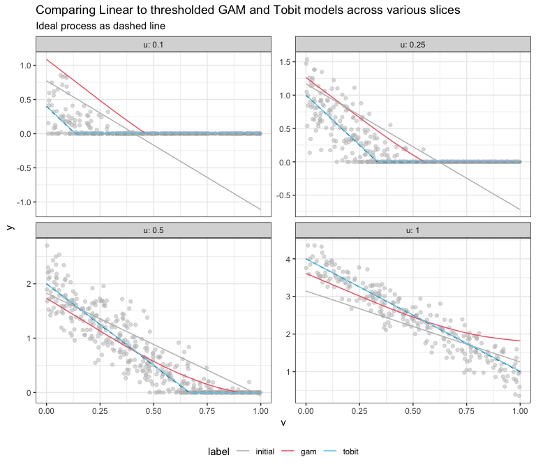
Conclusions #
For our original problem—post-hoc adjustments of an already established modeling procedure—a GAM adjustment seems to be the best way to adapt our modeling to higher-than-anticipated saturation frequency. However, Tobit adjustment is competitive. If you have the opportunity to design the modeling procedure de novo, GAM may not be the best option; though I admit, I didn’t spend any time trying to tune the model. If the process you are modeling is well-approximated as linear in the non-saturated region, then a thresholded Tobit model appears to be a good choice.
Obviously, to fit a full model, one can try many more methods: Poisson regression, trees, MARS, boosting, random forest, and so on. A typical task for the data scientist is to try many plausible methods on the client’s data and pick the one that appears to be the best practical trade-off for the given client.
Statisticians generally use the word “censored” when talking about processes that threshold out to a minimum or maximum value (or both). Often, the assumption is that the measurements are censored because of limitations of the measurement itself: for example, you can’t track a subject for more than five years, so the longest lifetime you can expect to measure is 5, even if the subject lives for decades longer. Models like Tobit try to predict as if the data isn’t censored: they can predict a lifetime longer than 5 years, even though those lifetimes can’t be measured.
I am using the word “saturated” to indicate that the outcome being measured literally cannot go beyond the threshold: counts can never be negative. A possibly useful analogy is the image from a digital camera: too much light “blows out” the photo. If you are trying to predict the intensity of the light that hit the camera sensor using the image pixels as the outcome data, then the data is censored. If you are trying to predict the values of the pixels, then the data is saturated. ↩︎